Learning from Prediction 2: Word Embeddings

<p class="kicker">GRA 4164 · Lecture 6 · Fall 2026</p>

## Learning from Prediction 2:<br>Word Embeddings

### Leif Anders Thorsrud & Vegard H. Larsen — BI Norwegian Business School

---

*"You shall know a word by the **company it keeps**."*

— J.R. Firth, 1957. Today we make that math.

---

## Where we are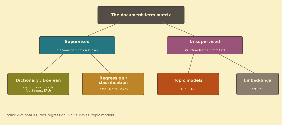

![Taxonomy: supervised and unsupervised methods on the document-term matrix](../figures/bow-methods-map.svg)

---

## What bag-of-words can't see

- In the document-term matrix, "good" and "great" are **unrelated columns**
- Word **order** gone, word **similarity** gone
- Embeddings: every word becomes a **dense vector** — similar words, similar vectors

---

## The picture to keep

![Toy 2D embedding: royalty and gender clusters, and king minus man plus woman approximately queen](../figures/embedding-toy.svg)

---

## Route one: counting

---

## Count the company: co-occurrence

- Slide a window of ±$b$ words (say $b = 4$) through the corpus
- $Co\_{ij}$ = how often word $j$ appears in word $i$'s window
- A $p \times p$ **word–word matrix** — words in rows *and* columns

---

## From counts to association: PMI

$$M\_{ij} = \log\_2\!\left(\frac{p\_{ij}}{p\_i \, p\_j}\right) \qquad \tilde{M}\_{ij} = \max(M\_{ij},\, 0)$$

- Together **more than chance** → positive; "the" next to everything → ≈ 0
- Keep only positives: **PPMI** (negatives are noisy)

---

## Shrink it: SVD, again

$$\tilde{M} \approx \underbrace{U\_{1:K} S\_{1:K}}\_{\text{embeddings } (p \times K)} \; V'\_{1:K}$$

- Truncated SVD — **the lecture-3 move**, applied to the word–word matrix
- Each **row of $U S$** is a word's $K$-dimensional embedding

---

## It works: 223 SOTU speeches

![Real PPMI plus SVD embeddings of State of the Union text showing war, money, law, and nations clusters](../figures/sotu-embeddings.svg)

---

## Route two: predicting

---

## word2vec: the game changer

- Mikolov et al. (2013): **learn** embeddings by prediction
- **Skip-gram**: predict the context words from the target
- **CBOW**: predict the target from its context
- Self-supervised — the sliding window labels the data, like lecture 4

---

## A two-layer network, no frills

$$h = W^1 x \qquad y = \text{softmax}(W^2 h)$$

- $x$: one-hot word (length $p$) — so $h$ is just **a row of $W^1$**
- $W^1$ ($K \times p$) is the **prize**: the embedding matrix
- No activation, no biases — simpler than lecture 4's MLP

---

## The trick: negative sampling

- Softmax over $p$ = 100k words every step — **too slow**
- Instead: logistic regression on pairs — real context → 1, random words → 0

$$L = \log \sigma(\vec{w}\_t \cdot \vec{w}\_c) + \log \sigma(-\vec{w}\_t \cdot \vec{w}\_{nc})$$

- 2–5 negatives per real pair, drawn $\propto \text{count}^{0.75}$

---

Counting and predicting land in **the same place** — again.

Levy et al. (2015): word2vec ≈ implicit PMI factorization.

---

## After word2vec

- **GloVe** (2014) — factorise global co-occurrence directly
- **doc2vec**, Word Mover's Distance — documents via embeddings
- The real limit: **one vector per word** — "apple" the fruit = "Apple" the firm
- Fixing *that* needs context-dependent embeddings → **lecture 8**

---

## What embeddings buy you

---

## Measure culture: Kozlowski et al. (2019)

- Build a **class dimension**: $\vec{rich} - \vec{poor}$, averaged over word pairs
- Project words onto it — and track **decades** of text
- Your reading: how "education", "leisure", "taste" moved along class over a century

---

## Measure risk, measure exposure

- **Labonne (2023)**: $\cos(\vec{recession} + \vec{risk},\; \vec{credit} + \vec{leverage} + \vec{funding})$ per month of news → a credit-sentiment index
- **Kapfhammer et al.**: climate-transition risk for commodity currencies from embedding arithmetic

Concept = sum of word vectors; index = cosine similarity.

---

## In sum

- Words become **vectors**; similarity and direction carry meaning
- **Counting route**: window co-occurrence → PPMI → SVD
- **Predicting route**: skip-gram + negative sampling; $W^1$ is the prize
- The two **agree** — and one vector per word is the limit transformers break

</div>

---

## Questions

## PPMI worked example (J&M)

| $Co$ | computer | data | pinch | result | sugar |
|---|---|---|---|---|---|
| apricot | 0 | 0 | 1 | 0 | 1 |
| digital | 2 | 1 | 0 | 1 | 0 |
| information | 1 | 6 | 0 | 4 | 0 |

- E.g. $\tilde{M}\_{\text{information,data}} = 0.57$ — but $\tilde{M}\_{\text{apricot,pinch}} = 2.25$
- **Rare pairs get extreme values** → smooth (add-one / add-two) before trusting

## Neural nets, the 60-second recap

- Unit: $z = w x + b$, activation $a = f(z)$ — sigmoid, or **softmax** for outputs
- Layers: $h^{l} = f(W^{l} h^{l-1} + b^{l})$ — features feeding features
- Trained by **gradient descent + backpropagation** on a loss
- Reference: Nielsen, *Neural Networks and Deep Learning* (free online)

## The embedding family tree

- **Count + factorise**: LSA cousins, PPMI + SVD
- **Predict**: word2vec (skip-gram, CBOW), GloVe in between
- **Contextual**: ELMo → BERT → GPT — one vector per word **per sentence**
- Today's methods are the ancestors of every LLM's input layer

---

## What's next

- **Lecture 7 (Mon):** large language models and tokenization — the LLM block begins
- **Before then:** finish the **Kozlowski et al. (2019)** reading
- Reading: J&M chapters 5 and 6